Highlighting my experience during coding of Stochastic Gradient Descent algorithm
olor:#ffffff;font-family:arial,tahoma,helvetica,freesans,sans-serif;">
Stochastic Gradient Descent is an online classification algorithm. This algorithm proves to be very efficient in classification of huge big data problems. Unlike Logistic
algorithm, which is somewhat ancestor of this, it takes one row at a time from the input data which can also be called as tuple instead of a whole matrix. The data possess by the tuple undergoes computation and result gets added to previous computed record.
There is a huge possibility of the usage of this algorithm in Big data analytics. Most common use case has been seen in medical field wherein the system accepted input from the patient on basis of cholesterol level and other parameters, and
with help of this algorithm gave a probability of that individual having heart disease. link
Through this blog I intent to share my team’s experience in coding this feature, as well as documenting major findings during course of time.
It was pretty difficult for us to find any c# code for the same algorithm. Initially Accord.net proved to be of some help http://code.google.com/p/accord/ related to Logistic learning, but
it didn’t have any help related to SGD which was our objective.
Nevertheless, we found some help from few articles and Java implementation of SGD in Apache Mahout. After much learning we had enough data to code in .net technology and came up with following findings.
1. We coded for Online Stochastic gradient using lazy stochastic method, which was easier to implement.
2. We calculated for Probability per epoch, log likelihood per epoch, error gradient and learning rate.
3. Input File Format:
For verification of result we took input csv file as
A,B,C,D,E,F
a,1,2,4,6,4
b,1,4,3,6,4
c,1,7,2,6,4
d,1,2,5,6,4
e,0,9,8,6,4
f,1,1,6,6,4
f,0,1,6,6,4
f,1,1,6,6,4
e,0,9,8,6,4
f,1,1,6,6,4
f,1,1,6,6,4
f,1,1,6,6,4
f,0,1,6,6,4
f,1,1,6,6,4
f,1,1,6,6,4
f,1,1,6,6,4
f,1,1,6,6,4
f,1,1,6,6,4
…
Note here, the dependent column is B and C,D,E,F are the independent column. Let me portray a scenario for better understanding. Assuming the first row(epoch) is having a patient entry. You can read this row as
a,1,2,4,6,4
· person name – a
· Having heart disease – yes or 1
· Cholesterol level above normal – 2
· Blood pressure -4 etc.
As you can see the dependent column had binomial values 0 or 1.
If you take a note of the pattern I have deliberately made the 4th multiple row to be 0 so that I get a probability of 0.75 (3 cases out of 4 are having heart disease). I had approximately 630 data with such entry.
4. Output File Format
The output that we achieved was in this format:
Result for per row,ProbabilityLikelihood,log likelihood, Error Gradient,Learning Rate
1,0.5,-0.693147180559945,0.5,15.8113883008419
1,1,0,0,15.0604916616593
1,1,0,0,14.4049036500379
1,1,0,0,13.825943979561
1,0,-100,-1,13.3096899721724
1,4.81619553731958E-190,-100,1,12.8455237353312
….
Resultant Headers for LR Classifier: Total Log Likelihood ,Deviance,Mean Error,Max Error
Result,-3987.86477761697,7975.72955523393,-0.000287308070520634,1
To us this huge output file was making no sense. As this was having a csv format we thought to depict graphical charts out of this.
Surprisingly, we got unique continuous patterns for the above outputs
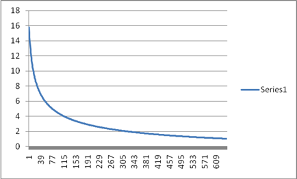
Learning Rate
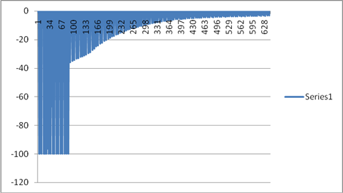
Log Likelihood
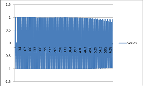
Probability

(Approximately coming to 0.75)
Error
Summary
Now after going through the charts the accuracy of the results were verified. Learning had an exponential decay, Log Likelihood was tending to zero, Probability was tending to 0.75 and error rates also were started to converge. Given a huge data of almost 1TB,
may be the observation would have shown more clear patterns till saturation limit.
I would like to acknowledge Ceaser Souza discussing with whom really v style="color:#222222;font-size:13px;line-height:18px;background-color:#ffffff;font-family:arial,tahoma,helvetica,freesans,sans-serif;">
Summary
Now after going through the charts the accuracy of the results were verified. Learning had an exponential decay, Log Likelihood was tending to zero, Probability was tending to 0.75 and error rates also were started to converge. Given a huge data of almost 1TB,
may be the observation would have shown more clear patthelped us to deep dive in the problem statement.
Please feel free to post your view and suggestion to this.